

We have many works in excel which should be grouped and processed data . They are many options and tools to arrange data in different forms . In those tools , sorting is one of the best techniques in excel. Color sorting is one of the sorting Technics in which you can arrange some data in a manner .
They are few color sorting Technics that I am going to cover in this article , they are
- Data sorting with single color .
- Data sorting with font color .
- Data sorting with conditional formatting icons .
So, the first one,
Sorting with Single Color
This is better Technic if you have only one requirement of grouping data .
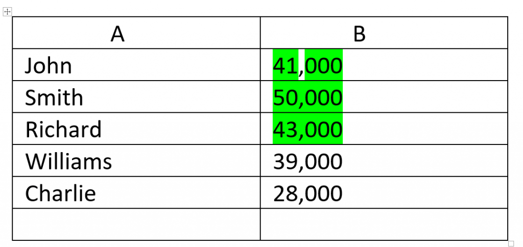
If we have the data table which shows us the salaries of company’s employees .
Then, if we use single color sort, then it will show like the above figure . .
Step 1) : Select the “ Data ” option which is at the top and then click on the “ Sort “ .
Step 2) : Then keep the mark ticketed in the box tilted “ My data has headers “ . You can also leave this without tick if your data doesn’t contain any headers .
Step 3) : Now, choose the option “ Sort by” and then select the “ Marks “ .
Note :
Here ,we have the data about a company’s salaries and names of the employees .So, we can use this Marks option as same because ,we will put salaries in the place of marks and names remains as same .
Step 4) : Then , select “ Cell Color “ in the middle box titled as Sort On .
Step 5) : And finally, choose colors from the order drop down menu . Sometimes ,it only contains green color . Select it .
Step 6) : Select the type position of the sorted data . If you select “On Top” , then all colored data will be sorted at the top of the table .If you select any other position ,then the data will sorted to there . Means, this specifies the colored/sorted data .
Click on the “ OK “ finally . If we need the salaries more than 40,000 in sorted data, then the figure 1 will be sorted as below after selecting OK .
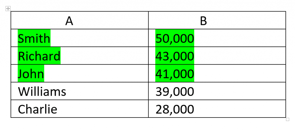
This type of sorting gathers the same colored items to a place and uncolored items will remain same.
2) Sorting with font color
This sorting also pretty good one but many don’t prefer to do this . This takes very simple techniques to be sorted .
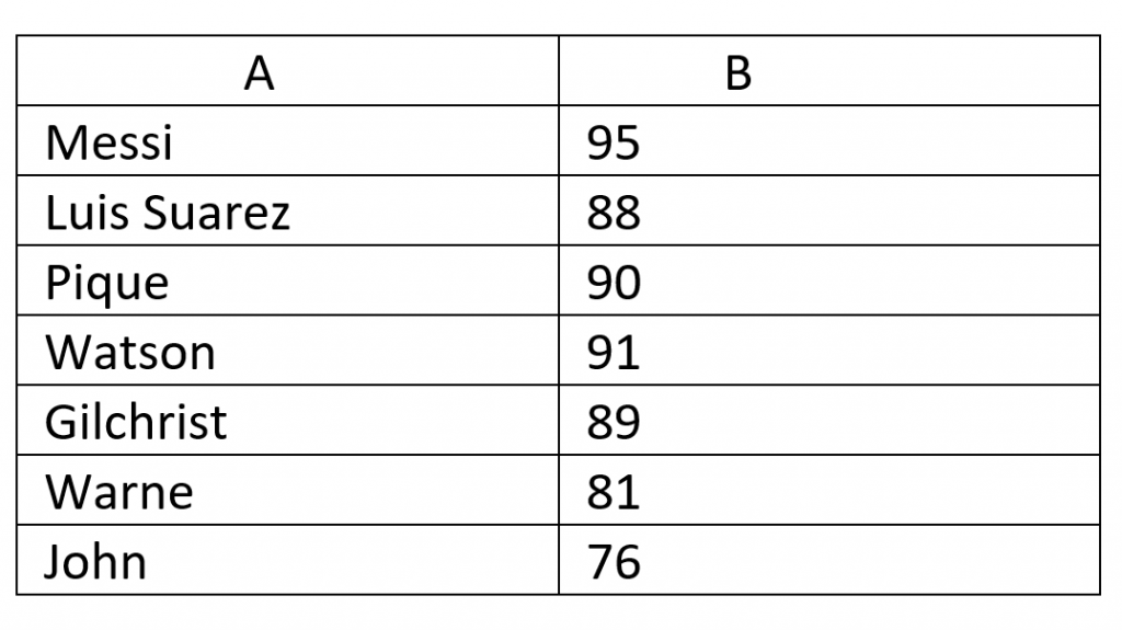
To discuss this method , let’s consider some students with their marks…
Step 1) : Select the “ Data ” option which is at the top and then click on the “ Sort “ .
Step 2) : Then keep the mark ticketed in the box tilted “ My data has headers “ . You can also leave this without tick if your data doesn’t contain any headers .
Step 3) : Now, choose the option “ Sort by” and then select the “ Marks “ .
Step 4) : Then , select “ Cell Color “ in the middle box titled as Sort On .
Step 5 : And finally, choose colors from the order drop down menu . Sometimes ,it only contains green color or red color . Select it .
Step 6) : Select the type position of the sorted data . If you select “On Top” , then all colored data will be sorted at the top of the table .If you select any other position ,then the data will sorted to there . Means, this specifies the colored/sorted data .
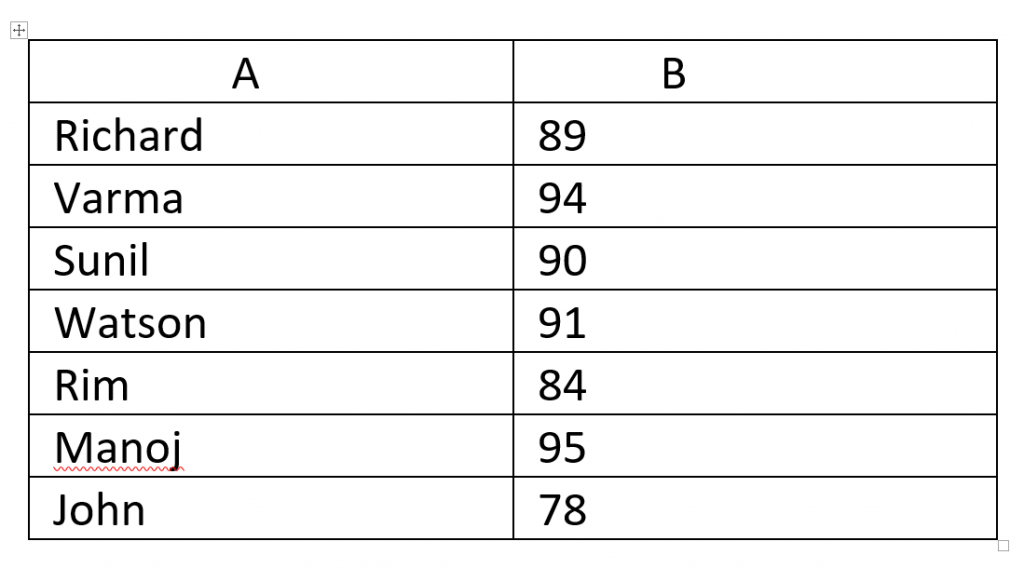
The lowest marks will be at the bottom like if we put below colored then ,those marks will be arranged at bottom .
Then, click on OK to get the sorted table . .

So, this method arranges the font colored and uncolored values in ascending and descending order at wherever position we want…
3) Sorting with conditional formatting Icons
This type of sorting make visuals clear and obvious to the reader .
This adds a layer with new icons on the sorting is based on .
Let’s consider set or table of data .
Here are the steps for understanding the process ,
Step 1) : Select the “ Data ” option which is at the top and then click on the “ Sort “ .
Step 2) : Then keep the mark ticketed in the box tilted “ My data has headers “ . You can also leave this without tick if your data doesn’t contain any headers .
Step 3) : Now, choose the option “ Sort by” and then select the “ Marks “ .
Step 4) : Then , select “ Conditional Formatting” in the middle box titled as Sort On .
Step 5) : And finally, choose colors from the order drop down menu . Sometimes ,it only contains green color . Select it .
Step 6) : Select the type position of the sorted data . If you select “On Top” , then all colored data will be sorted at the top of the table .
Step 7) : Select the option “Add Level Button “.
Note : Do this same three times by selecting green, red and yellow respectively . And again “Marks” and then “Conditional Formatting” .
The table contains circles with colors as our assignments . If we assign red for low marks , green for highest marks and yellow for average marks. Then they’ll be arranged in order .
Then, click on OK to get the sorted table . .
See Also…
3 Ways to remove unwanted characters from Excel(Opens in a new browser tab)